We summarize here the two capabilities of the program.

Pressure drop calculation for pipe networks including fittings and flare nozzles.

We summarize the relationships for pressure drop in

• pipes,
• expansions and contractions,
• bends
• junctions
• fittings

We also give the design options that we provide.

1) Pipes.

The fundamental equation for pressure-drop in pipes is

(1/a) (G/A) ² ln(v ₂ / v ₁ ) + W + 4f _m (l/d)(G/A) ² =0    (Where dW = MdP/ v)      (1)

a allows for the velocity profile in the pipe (for turbulent flow, it is about 0.94).
G is the mass flow through the pipe
v is the molar specific volume; v ₁ and v ₂ are the specific volumes at inlet and outlet
M is the mean molecular weight of the mixture
f _m is the mean friction factor
l is the pipe length
d is the pipe diameter

Equation (1) applies for gas, liquid and two-phase flows. It also applies for isothermal and adiabatic flows.

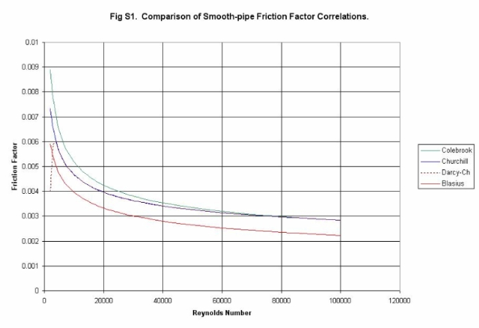
For liquids and vapours, friction factor varies very little with distance along the pipe. However, for two-phase flows, friction factor depends strongly on pressure. The correct choice of mean is then essential for computing the frictional pressure drop accurately. To good approximation, the same mean applies for single-phase flow and two-phase flow. The user has the choice of Colebrook, Churchill, Darcy-Churchill and Spitzglass friction factor correlations. Figure S1 compares the computed friction factors for smooth pipes. It also shows the friction factor computed by the Blasius Equation, which is the most accurate for smooth pipes. It is seen that there is an 18% spread between the estimates. This spread gives an estimate of the intrinsic error in estimating turbulent pressure drops. Smooth pipe conditions are very well defined. Rough pipes are less well defined, and we may expect larger errors in estimated friction factors. Flaresign aims to solve pressure drop equations to within 2% to 3%. We see that this precision is an order of magnitude better than the intrinsic accuracy of the equations that we are solving.

The relationship between P and v depends on the fluid, and for gas and two-phase flows, on the heat flux conditions (isothermal, adiabatic or finite flux). Using the Chemcept Pressure-Virial Equation of State, the integral term in Equation (1) reduces to:

dP/ v = PdP/ [F ₁ {T} + F ₂ {T}P]          (2)

Equation (2) applies to both single phase and two-phase flow. For isothermal flow, there is a simple analytical solution.

For adiabatic (or finite heat transfer) flow, temperature is related to pressure by energy balance. Flaresign estimates temperatures at every node on the network from which, for each pipe length, it approximates the relationship between T and P. The equations can then be solved analytically. The temperatures at each node are recomputed by energy balance and a super-linear iterative scheme is employed to reach converged estimates of the temperatures. The adiabatic option is not available in the current release.

The accuracy of the analytical solutions can be appreciated by the following examples:

Single phase isothermal flow of ethylene gas at 298 K
Mass Flow Rate 100 kg/s
Discharge directly to atmosphere at 1.0 bar
Pipe Length = 10 km
Pipe Internal Diameter = 0.7 m
Pipe Roughness = 0.04572 mm
Colebrook Friction Factor Formula.

The 1-step analytical solution is compared to an accurate numerical solution in Table 1

Table 1. Flow of Ethylene Gas in 10-km pipe.

			Pressure in (bar)	Pressure out (bar)
Numerical Solution		9.86708	1.00129
Analytical Solution		9.86669	1.00129
                      

It is seen that the analytical solution differs from the accurately computed solution by only 0.004%. This difference is negligible for a calculation that probably has intrinsic errors of 10%. Furthermore, few numerical integrations will be converged this accurately. Note that the pipe shows almost a factor-of-ten pressure drop. Such a large pressure ratio in one pipe can occur in emergency release networks, but is unusual. Over 45% of the pressure drop is in the last 25% of the pipe length. Thus, the remaining 75% of the piping could use a smaller diameter with negligible increase in overall pressure drop. A smaller pipe is possible because, although the output to the large pipe is 80% choked, the inlet is only 8% choked. Furthermore, at 75% of the length, the pipe is still only 15% choked. Thus, there is a large velocity margin before choked conditions are approached. There would be cost benefits in smaller pipe and an increased safety margin because of the higher pressures than can be safely held in a smaller diameter pipe of a given gauge. For these reasons, it is unlikely that practical applications will show a greater proportional pressure drop in one length of pipe. The result confirms that the analytical solution gives excellent accuracy as well as several orders of magnitude decrease in computer run-time.

The approximation is less accurate for 2-phase flow because the two-phase friction factor varies strongly with mixture pressure. Thus, the choice of mean friction factor in equation (1) becomes more critical. Table 2 gives a comparison of accurate and approximate 2-phase pressure drop computations. The two-phase calculation is for the same conditions as for the single-phase calculation except that the gas flow is reduced to 50 kg/s and a liquid water flow of 50 kg/s is introduced.

Table 2. Flow of Ethylene water mixture in a 10-km pipe.

			Pressure in (bar)	Pressure out (bar)
Numerical Solution		13.99070		1.00018
Analytical Solution		13.93840		1.00018
                      

(The difference between the outlet pressures and the single-phase outlet pressures arises because we insert a hypothetical zero pressure drop KO drum. The resulting reduced gas flow has a lower pressure drop as it is discharged to atmosphere).

The resulting error in using the approximate analytical solution is 0.4%. This error is small compared to the inherent error in two-phase flow friction-factor correlations. These errors are typically 20%. Both the Dukler method and the Lockhardt-Martinelli method show similar accuracy (or lack of it). We use a modified Lockhardt-Martinelli method because it has the benefit of giving an upper-bound estimate of the two-phase friction factor within the accuracy of the single-phase friction factor methods employed. Thus, the user can be assured that the pressure drop is not underestimated.

As for the single-phase example, the example probably illustrates extreme conditions, not likely to be met in practice. Thus, over 50 % of the pressure drop is in the last 25% of the length. At the exit of the pipe, the flow is 56% choked, but is only 7% choked at the inlet to the last 25%. For a given mass flow rate, two-phase friction factors increase as the pressure drops (roughly as the inverse square root of pressure). Thus, pressure drop is forced into the low-pressure section of a pipe even more than is the case for single-phase flow. There is then a stronger incentive to have larger diameter pipes at the low-pressure end and smaller diameter pipes at the high-pressure end. For shorter pipes, the analytical solution gives much closer agreement with an accurate numerical integration. Thus, the discrepancy of 0.4% is unlikely to be exceeded in any practical application.

2) Sonic and Choking Flow.

The maximum velocity that can be achieved in a uniform pipe is the choking velocity. For the adiabatic flow of a single-phase gas, the choking velocity is the sonic velocity. Flaresign gives solutions of equation�(1) that are less than the choking velocity for all single- and two-phase flow regimes. However, it is desirable to be able to compute the choking velocity to ensure that networks are not designed to get close to the choking velocity in pipe flow. Choking conditions can also arise in pipe fittings and at pipe expansions. Thus, we need to be able to compute choking flow for any fluid.

For flow in pipes, Whalley shows that the liquid velocity can be treated as the same as the gas velocity for inertial calculations. This assumption may be incorrect in computing hold-up. However, the total kinetic energy of the liquid is the same as if it were flowing at the same velocity as the liquid. Changes in hold-up and radial flow distribution compensate through the different flow regimes maintain the inertial identity. Sudden accelerations and decelerations may occur in fittings, and cause the liquid velocity to change relative to the gas. However, we assume that we can maintain the identity in order to compute two-phase choking flow.

The basic thermodynamic equation for choking flow can be derived from equation (1). For uniform flow across the pipe, it is:

u _X = v[-v ² (dP/dv) _X /M]          (3)

In equation (3), u is velocity; the other symbols are as for equation (1). Subscript "X" specifies what is held constant. Thus, for isothermal flow "X" is temperature, for isentropic flow, "X" is entropy. The Chemcept 2-phase equation of state enables equation (3) to be solved analytically for conditions of practical interest. A number of competitive programs assume that the compressibility factor, Z , remains constant when the partial differential is calculated. Flaresign employs a full equation of state so that dZ/dv is automatically computed. Thus, Flaresign provides a more accurate estimate than some systems that employ more complex physical-property correlations.

Flaresign corrects equation (3) to allow for radial velocity profile.

3) Expansions and Contractions.

Flaresign is one of very few systems that has a theoretically consistent treatment for the flow of compressible and two-phase fluids through fittings.

There are well-established correlations for liquid flow pressure-drop through fittings. These same correlations are applied to gas flows with low pressure-drops (when compressibility effects can be ignored). There have been a limited number of publications showing that the correlations cannot be applied when there is a gas flow with significant pressure drop. (See for example, the early work by Benedict, Carlucci and Swetz).

We consider first sudden expansions. For an incompressible fluid, a simple momentum balance gives an excellent estimation of pressure change. Theoretically, the incompressible formula should not apply to a compressible fluid. When pipe diameter increases, the fluid velocity falls and the pressure increases. For a compressible fluid, the increase in pressure gives a decrease in specific volume so that the velocity falls further. The further fall in velocity gives rise to a further increase in pressure. It is possible to consider these effects in performing a modified momentum balance across a sudden pipe expansion. The resulting expression correlates the data of Benedict and co-workers better than their original correlation. This modified formula is employed in Flaresign. It has the benefit that, at low pressure-drops, it automatically reduces to the incompressible flow formula. We have access to no experimental data for high-pressure gases when non-idealities become important. However, our simple theory accounts for the data we can find. Accordingly, we have used the Chemcept-data equation of state to extend the method to non-ideal gas flows. With slightly less justification, we also apply the method to two-phase flows through pipe expansions. A theoretical treatment indicates that the resulting error should be small. The resulting expressions reduce to the incompressible formula for 100% liquid. Thus, we have the benefit of a single simple method that applies equally to ideal and non-ideal gases, to liquids and to gas/liquid mixtures.

For contractions, we adopt the model that the fluid accelerates reversibly to a vena-contracta from which it expands irreversibly to the new (reduced) pipe diameter. The pressure gain in the expansion step is treated exactly as the expander model. The pressure drop in the reversible acceleration is obtained by solving the flow equations using the Chemcept-data equation of state. Again, the resulting correlation reproduces the Benedict et al results better than their own correlation. It has the benefit of automatically reducing to the incompressible fluid model under limiting conditions.

As in all its other models, Flaresign corrects for turbulent radial velocity profile.

4) Fittings with one inlet and one outlet.

Flaresign treats all such fittings as having the same size inlet pipe and outlet pipe. Where there is a difference, an additional expander or contractor must be added to the simulation. There are three ways of modelling these fittings. First, they can be modelled using K-values (the "velocity head" method). Secondly, they can be modelled using an "equivalent pipe length". Thirdly, they can be modelled as a K-value plus a pipe length. This third method is the most reliable if the parameters are known. The K-value method is better than the equivalent pipe-length method. Flaresign allows all three options. Flaresign also allows the option of automatically converting all K-values to equivalent lengths or vice-versa.

For the K-value method, Flaresign uses a modification applicable to compressible and to multi-phase fluids. Published K-values are derived from tests with incompressible fluids. Theoretically, the K-value is derived from relationships representing the acceleration and deceleration of the fluid through the fitting. For example, excellent estimates of K-values for bends can be derived by recognizing that the fluid is decelerated in its original flow direction. Consequently, the pressure is higher in the direction-change zone. The fluid is then accelerated in its new direction. Mathematically, the pressure drop calculation is identical to the calculation for an expansion followed by a contraction. Thus, as for expansions and contractions, we would expect the pressure drop for compressible fluids to be given by a modified formula. The point of highest pressure will be a point of lowest velocity and highest density. At the low-pressure outlet, the density will be less, and hence the velocity higher. The overall pressure-energy loss is then greater than for an equivalent incompressible fluid. To allow for compressibility, K-values are converted to equivalent area changes. In accordance with theory, for incompressible fluids, Flaresign gives exactly the same pressure drop as for the equivalent K-value. For compressible and two-phase fluids, a higher pressure-drop is estimated.

Fittings such as valves operate by restricting the flow and then letting it expand. Thus, the flow accelerates to the narrowest opening (or vena contracta, where that is smaller) from which it then decelerates to the outlet. For such fittings, the K-value is used to estimate an equivalent area, which, in contrast to the bend area, is smaller than the pipe area. The fitting is modelled as a reversible acceleration to the constriction followed by an irreversible deceleration. For incompressible fluids, this model gives the same pressure drop as the K-value model. However, for compressible fluids, it gives a wider pressure excursion, and hence a larger pressure drop. The model applies also to non-ideal gases and two-phase flows. Sonic or choking flow frequently arises in fittings. Flaresign checks for choking/sonic flow and gives a higher pressure-drop if choking conditions are reached. Flaresign also checks for liquid cavitation in flow through fittings and gives a higher pressure-drop if it occurs. (This correction is approximate in the current version because gas solubility and vapour pressure is not accurately computed).

Note that the pressure drop in fittings is primarily an inertial effect from alternate acceleration and deceleration. The equivalent pipe-length method relies on friction factor being insensitive to pipe diameter and Reynolds Number. None of the equivalent pipe-length methods is accurate, and none more accurate than that used by Flaresign. The equivalent pipe-length employed in Flaresign is satisfactory within � 40% for single-phase flows. When the disposition of fittings is unknown in the early design stages, this accuracy is satisfactory. However, two-phase friction factors can be more than an order of magnitude greater than single-phase friction factors; they are also sensitive to pressure. Thus, unless you know the pressure, flow rate and pipe diameter in advance, it is difficult to assign an equivalent pipe length for 2-phase flow through a fitting. Flaresign has a modified method for estimating equivalent pipe-length that is normally within a factor of two, but can be a factor of four in error. Such errors are normally acceptable when total fitting pressure drop is a small fraction of the total. However, bear in mind that, in a flare network, the total pipe-length equivalent to fittings can amount to several hundred metres. On balance, it is better to use K-values when they are available. Flaresign provides the most comprehensive range of K-value based tools for handling non-ideal and two-phase flow through fittings.

The Spitzglass equation is now mainly of historical interest, but is still included in some current regulations. It employs a smaller equivalent pipe length appropriate to the smaller gas pipe sizes that were current when it was developed almost a century ago. Flaresign allows the method to be used at any pressure for any single-phase or two-phase flow. However, application should be restricted only to low pressure gas pipelines.

5) Junctions.

For most junctions, the area of the pipes entering the junction exceeds that of the single pipe leaving the junction. This situation is always the case if one of the inlets (typically the straight-through inlet) has the same diameter as the outlet. Flaresign divides the outlet area into two parts, one corresponding to each inlet flow. The division is arranged such that both inlet streams come to the same velocity as they are mixed in the outlet pipe. Normally, both inlet streams are accelerated to reach a common outlet velocity. In such cases, Flaresign treats the two inlet streams as both entering area reduction fittings. The program also caters for the cases when the relevant areas increase or remain the same (which can happen, for example, if one inlet has no flow). The relevant inlet is then treated as an expansion. Equally, it may be that one inlet stream accelerates and the other decelerates. The total fitting pressure-drop comes from combining area-change and direction-change effects. The user can apply a K-value and/or an equivalent length (to estimate direction-change pressure-drop). Thus, Flaresign provides a junction modelling facility that is based on sounder science than most of its competitors.

6) Knock-out drums.

Knock-out drums provide liquid/gas separation by a combination of settling and inertial impaction resulting from sudden changes in gas flow direction or centrifugal force. The balance of mechanisms depends on the design of the particular separator. Flaresign provides a simple modelling capability which assumes that gas and liquid are separated with 100% efficiency. Pressure drop is computed based on changes in direction, which are modelled as equivalent to expansions and contractions. The sequence of direction changes is represented by a single equivalent area. A facility is provided to compute this equivalent area from calibration data, namely one or more pressure drops for known flow conditions.

7) Flares.

Flaresign computes the pressure drop through a flare tip assuming adiabatic discharge of the gas to atmosphere. The adiabatic pressure drop (and temperature drop) is computed from the equation of state also allowing for change in Heat Capacity Ratio as the gas expands. Each flare tip is characterized by an equivalent discharge area. A facility is provided to compute this area from Manufacturer's calibration data (flow versus pressure for a known gas mixture and known inlet temperature).

Flaresign provides protection against a failure in the unlikely circumstance of choked flow from an open pipe. Sonic discharge from an open pipe is greater than the choked flow in an isothermal pipe. If a user specifies isothermal flow with discharge from an open pipe at a sufficiently high Mach Number, the flow would be greater than the maximum possible flow in the pipe. It would then be impossible to solve equation (1). Such an unlikely failure is eliminated by limiting the flow in the pipe feeding a flare nozzle to its choked flow. Such detailed attention to potential error conditions ensures that Flaresign is resistant to run-time failure.

8) Design Options.

Flarenet provides the following design options:

• 1) Simulation of specified flow network with fixed outlet pressure and adjustable inlet pressures.
• 2) Design to give a maximum specified fraction of choking flow at any point in the network.
• 3) Design to give a maximum specified velocity at any point in the network.
• 4) Design to give a maximum specified velocity head at any point in the network
• 5) Design so that no specified inlet pressure is exceeded.

Flame Shape and Radiation Calculations.

Flaresign offers the following calculations:

1) Flame length and 3-dimensional axial trajectory.
2) Flame lift-off (distance between flare tip and start of combustion zone).
3) Flame diameter at flame base (adjacent to flare tip) and flame tip (remote from flare tip).
4) Heat generated by combustion and stoichiometic air consumed.
5) Proportion of heat generated that is radiated.
6) The radiation intensity on a surface inclined to the flame.

The methods used are as follows:

1. Flame length and shape.

1) API RP 521-1968*
2) Brzustowski Method*
3) GKN Birwelco Method*
4) Kaldair Method*
5) Shell Method*

NOTE: * We use these titles to identify the methods. We do not guarantee that we have correctly interpreted the publications on which our code is based. None of the companies or individuals named have endorsed our implementations. Some of the methods apply to proprietary flare tip designs, and may not apply exactly to other designs. All methods have been abstracted from publications in the public domain, and most have been modified by ourselves. We believe that our implementations give a good preliminary-design basis but, particularly where proprietary flare tip designs are used, tip manufacturers should be consulted to fine-tune the calculations.

We summarize here some of the features of our implementation.

We employ an analytical integration of the API method.

The Brzustowski method, as published, shows a number of problems. First, it gives infinite length flames in zero wind speeds. For wind speeds above about 1 m/s, it gives a shorter flame than the API flame. When the user selects the Brzustowski option we compute both the Brzustowski and API flame lengths and return the shorter of the two. Secondly, it includes a conditional expression that, for an infinitesimal change in fuel flow rate, can give rise to a sudden change in radiation intensity of over 25%. The correlations are modified so that, at the conditional break, both expressions give the same answer, which is the geometric mean of the two Brzustowski answers. For higher and lower values, the modified correlations asymptotically approach the unmodified Brzustowski values. Thirdly, the Brzustowski correlations are in terms of the horizontal projection of the flame. All other flame shape correlations are in terms of the axial distance along the flame. Consequently, the "mid-point" of the Brzustowski flame is not the mid-point of the axis of the flame. The distance along the axis varies with flare and wind conditions. This anomaly makes it difficult to modify the Brzustowski flame in order to calculate line and surface source radiation. For consistency with other flame models, we compute all distances along the axis of the flame, rather than the horizontal projection of the flame. The computed radiation intensity increases slightly because the mid-point of the axis is nearer to the flare tip than is the point corresponding to the mid-point of the horizontal projection.

The flame shape equations recommended by GKN Birwelco authors includes a term for "uplift velocity". The velocity corresponds to the vertical convective velocity at the flame tip. We compute that velocity from simple theory. However, we believe that GKN Birwelco use an experimentally determined value that is, in effect, an empirical correction to give a good match with observed flame shapes. Their equations also include a factor "f" for which they give no guidance. We calculate a theoretical value based on momentum balance. Finally, they have a condition under which effective flare-tip discharge-velocity is brought to zero. Their published equation gives an illogical large velocity jump for a minuscule change in wind speed. We have modified the condition so that our equation behaves similarly, but does not exhibit the illogical jump. We integrate their equations numerically.

We have empirically correlated the data published by McMurray (of Kaldair), so that flame length depends on heat release rate and Mach number. Thus, "supersonic" flares are shorter than subsonic flares. We employ their published analytical integration.

We have considerably modified the correlations published by Chamberlain describing the model based on extensive Shell data. The modifications should give minor differences under normal conditions, but behave more sensibly when extrapolated to unusual conditions. Thus, Chamberlain employs an approximate empirical relationship between mean molecular weight and stoichiometric air requirement. We use the Chemcept-data database that gives exact stoichiometric requirements for any mixture. For "supersonic" flares, Chamberlain presents equations for computing the hypothetical conditions (temperature, density, velocity, jet cross-sectional area etc) at which an expanding supersonic jet from a sonic flare tip reaches atmospheric pressure. We use a set of equations consistent with the equations we use in pipe network simulation. The result should be little different, but (for us) ensures consistency, maximizes code reuse and minimizes testing. Chamberlain presents equations that show the effect on flame length when a flare is tilted into or out of a wind. However, they show a dramatic difference in length when tilted into a wind of 0.00001 m/s and into a wind of �0.00001 m/s. We believe that the observed effect results primarily from a balance between buoyancy and inertial forces. Accordingly, we employ a modified formula that depends only on the orientation to the horizontal. For near-vertical flares, it gives results almost identical to the equations presented by Chamberlain. Chamberlain presents equations for flame tilt as a function of wind speed and Richardson Number. The equations are clearly wrong for tilt angles of more than a few degrees. Specifically, they can show flames that tilt into the wind, horizontal flames that tilt downwards, and flames that tilt by more than 360 degrees. Flaresign employs a completely new set of equations. These equations are derived from a model in which flame velocity is resolved into three components at right angles, namely vertical, horizontal in the wind direction and horizontal normal to the wind direction. The resulting equations give very similar results to the Shell equations for tilts of less than 45 degrees. However, their asymptotic behaviour is sensible. Specifically, the asymptotic behaviour in very high winds is that the flame tilts in the direction of the wind and lies horizontal. All the equations have been modified such that they are in consistent SI units. Despite the large number of changes made, the extensive published experimental data probably make this model the most reliable.

2. Flame Diameter.

We require the flame diameter as a function of axial distance in order to compute the surface area of the flame. Chamberlain gives correlations for the flame base diameter and the flame tip diameter. To good approximation, flame diameter increases linearly with axial distance. The flame tip diameter correlation provides an excellent fit of extensive observations of full-scale flames. This correlation has been applied to all flame models. The correlation at the flame base is more scattered, but is less important in determining total flame surface area. The full published correlation has been applied to the Shell model, but a simplified correlation has been applied to the remaining four models.

Table 3. Data for Flame Length and Shape Computations.
Gas Flow	Tip Area	Discharge	Mach		Jet  Velocity	Jet  Temp	Heat Release
(kg/s)		(m2)		Pressure	Number		(m/s)			(K)		(MW)
				(bar)
Methane
	25	0.15		1.0000		0.5786		246.08			285.40		1250.70
	25	0.02		4.1419		1.7507		704.74			260.15		1250.70
	50	0.30		1.0000		0.5786		246.08			285.40		2501.40
	50	0.04		4.1419		1.7507		704.74			260.15		2501.40
	100	0.60		1.0000		0.5786		246.08			285.40	 	5002.80
	100	0.08		4.1419		1.7507		704.74			260.15	 	5002.80
n-Butane
	25	0.15		1.0000		0.3345		67.83			297.91		1142.96
	25	0.02		2.3732		1.7234		307.74			276.72	 	1142.96
	50	0.30		1.0000		0.3345	  	67.83			297.91	 	2285.93
	50	0.04		2.3732		1.7234		307.74			276.72	 	2285.93
	100	0.60		1.0000		0.3345	  	67.83			297.91	 	4571.86
	100	0.08		2.3732		1.7234		307.74			276.72	 	4571.86
                      

3. Comparison of Flame Length and Shape Calculations.

The five models are compared for twelve sets of conditions covering a light gas (methane), a heavy gas (butane) and both subsonic and supersonic flow. The flare tip conditions are summarized in Table 3, above. For all tests, the temperature of the gases entering the flare tip was taken to be 300 K. In adiabatic expansion, the gas cools in its passage through the flare tip. For supersonic flames, the gas cools further as the gases leaving the flare tip expand further. The cooled gas temperatures are reported in Table 3. Tables R1 to R4 summarize the flame length and orientation computations. They were performed for wind speeds of 0 m/s, 2 m/s, 10 m/s and 50 m/s. These speeds correspond to still air, 4.5 mph (light breeze), 22 mph (brisk wind), and 110 mph (extremely strong gale). For given conditions, the estimated lengths differ by about a factor of four. The differences may result in part from differences in flare tip design and in difficulty in defining flame length. The latter difficulty probably accounts for differences of �20%. There is also a difficulty relating to conduct of field trials. It is not possible to control wind speeds in conducting full-scale trials. Thus, most trials are conducted in the wind-speed range 2 m/s to 10 m/s. If we restrict the comparison to wind speeds of 2 m/s to 10 m/s, we get closer agreement. If we further restrict comparisons to results obtained from tests conducted by major oil companies, we get still closer agreement. Thus, if we focus on Brzustowski (trials conducted with Esso), Kaldair (trials conducted with BP), and Chamberlain (trials conducted by Shell), agreement is within the accuracy with which flame lengths can be estimated. The level of agreement with Butane is surprising because no large-scale trials have been conducted with this gas. For both gases, the agreement covers both flame length and the extent to which flames are deflected in the wind.

It may be surprising that such a level of agreement is achieved between models based on such different theory. Thus, Brustowski uses Lower Flammable Limit as a prime parameter, Kaldair uses heat release, and Shell uses stoichiometric oxygen requirement. In practice, for hydrocarbons, there is a strong correlation between these parameters. Thus, any flame length correlation in one parameter can be converted to a correlation in the other by substituting the relationship between the relevant physico-chemical properties.

Table R1. Flame Length and Shape: Subsonic Flow, Methane Gas.

Mass Flow (kg/s)	25.00	25.00	25.00	25.00	50.00	50.00	50.00	50.00	100.00	100.00	100.00	100.00
Wind (m/s)		0.00	2.00	10.00	50.00	0.00	2.00	10.00	50.00	0.00	2.00	10.00	50.00	
API R521
Flame Length (m)	74.71	74.71	74.71	74.71	103.77	103.77	103.77	103.77	144.13	144.13	144.13	144.13
Base Dia/Length	0.0205	0.0205	0.0205	0.0205	0.0208	0.0208	0.0208	0.0208	0.0212	0.0212	0.0212	0.0212
Tip Dia/Length	0.2597	0.3007	0.3978	0.4414	0.2597	0.3007	0.3978	0.4414	0.2597	0.3007	0.3978	0.4414
Height/Length	1.0000	0.8276	0.5610	0.2681	1.0000	0.8298	0.5645	0.2709	1.0000	0.8319	0.5681	0.2736
Deflection/Length	0.0000	0.3762	0.6824	0.8941	0.0000	0.3729	0.6792	0.8926	0.0000	0.3697	0.6760	0.8910	
Brzustowski	
Flame Length (m)	74.71	48.17	25.83	25.54	103.77	68.12	36.53	36.11	144.13	96.34	51.66	51.07
Base Dia/Length	0.0205	0.0318	0.0592	0.0599	0.0208	0.0318	0.0592	0.0599	0.0212	0.0318	0.0592	0.0599
Tip Dia/Length	0.2597	0.3007	0.3978	0.4414	0.2597	0.3007	0.3978	0.4414	0.2597	0.3007	0.3978	0.4414
Height/Length	1.0000	0.9868	0.7445	0.2736	1.0000	0.9868	0.7445	0.2736	1.0000	0.9868	0.7445	0.2736
Deflection/Length	0.0000	0.1132	0.5226	0.8920	0.0000	0.1132	0.5226	0.8920	0.0000	0.1132	0.5226	0.8920	
GKN Birwelco
Uplift Velocity-m/s	0.6678	0.4981	0.2846	0.2311	0.6923	0.5163	0.2951	0.2396	0.7177	0.5353	0.3059	0.2484
Flame Length (m)	63.19	63.19	63.19	63.19	87.77	87.77	87.77	87.77	121.91	121.91	121.91	121.91
Base Dia/Length	0.0242	0.0242	0.0242	0.0242	0.0246	0.0246	0.0246	0.0246	0.0251	0.0251	0.0251	0.0251
Tip Dia/Length	0.2597	0.3007	0.3978	0.4414	0.2597	0.3007	0.3978	0.4414	0.2597	0.3007	0.3978	0.4414
Height/Length	1.0000	0.5313	0.1932	0.0605	1.0000	0.5347	0.1937	0.0606	1.0000	0.5383	0.1942	0.0607
Deflection/Length	0.0000	0.7608	0.9383	0.9860	0.0000	0.7595	0.9383	0.9860	0.0000	0.7581	0.9383	0.9860	
Kaldair
Uplift Velocity-m/s	0.4777	0.3563	0.2036	0.1653	0.4952	0.3694	0.2111	0.1714	0.5134	0.3829	0.2188	0.1777
Flame Length (m)	45.32	45.32	45.32	45.32	62.35	62.35	62.35	62.35	85.76	85.76	85.76	85.76
Base Dia/Length	0.0337	0.0337	0.0337	0.0337	0.0345	0.0345	0.0345	0.0345	0.0355	0.0355	0.0355	0.0355
Tip Dia/Length	0.2597	0.3007	0.3978	0.4414	0.2597	0.3007	0.3978	0.4414	0.2597	0.3007	0.3978	0.4414
Height/Length	1.0000	0.9810	0.7797	0.3755	1.0000	0.9822	0.7870	0.3817	1.0000	0.9833	0.7942	0.3880
Deflection/Length	0.0000	0.1573	0.5319	0.8681	0.0000	0.1525	0.5239	0.8651	0.0000	0.1479	0.5159	0.8620	
Shell	
Lift-off (m)		14.07	8.75	3.66	0.79	18.94	11.77	4.89	1.06	25.47	15.82	6.53	1.41
Flame Length m	70.35	50.59	35.13	34.47	94.69	68.10	47.28	46.40	127.35	91.59	63.59	62.40
Base dia/Length	0.0062	0.0947	0.0996	0.0216	0.0065	0.0995	0.1080	0.0244	0.0069	0.1046	0.1167	0.0275
Tip Dia/Length	0.2597	0.3007	0.3978	0.4414	0.2597	0.3007	0.3978	0.4414	0.2597	0.3007	0.3978	0.4414
Height/Length	1.0000	0.9881	0.7990	0.3976	1.0000	0.9895	0.8175	0.4202	1.0000	0.9908	0.8346	0.4431
Deflection/Length	0.0000	0.1540	0.6014	0.9176	0.0000	0.1443	0.5759	0.9075	0.0000	0.1354	0.5509	0.8965

Table R2. Flame Length and Shape: Supersonic Flow, Methane Gas.

Mass Flow (kg/s)	25.00	25.00	25.00	25.00	50.00	50.00	50.00	50.00	100.00	100.00	100.00	100.00
Wind (m/s)		0.00	2.00	10.00	50.00	0.00	2.00	10.00	50.00	0.00	2.00	10.00	50.00	
API R521
Flame Length (m)	74.71	74.71	74.71	74.71	103.77	103.77	103.77	103.77	144.13	144.13	144.13	144.13
Base Dia/Length	0.0075	0.0075	0.0075	0.0075	0.0076	0.0076	0.0076	0.0076	0.0077	0.0077	0.0077	0.0077
Tip Dia/Length	0.2597	0.2858	0.3613	0.4497	0.2597	0.2858	0.3613	0.4497	0.2597	0.2858	0.3613	0.4497
Height/Length	1.0000	0.7564	0.4603	0.1977	1.0000	0.7591	0.4638	0.1999	1.0000	0.7619	0.4673	0.2021
Deflection/Length	0.0000	0.4736	0.7668	0.9307	0.0000	0.4701	0.7640	0.9296	0.0000	0.4666	0.7613	0.9285	
Brzustowski
Flame Length (m)	74.71	45.09	22.49	19.53	103.77	63.76	31.81	27.62	144.13	90.18	44.98	39.06
Base Dia/Length	0.0075	0.0124	0.0248	0.0286	0.0076	0.0124	0.0248	0.0286	0.0077	0.0124	0.0248	0.0286
Tip Dia/Length	0.2597	0.2858	0.3613	0.4497	0.2597	0.2858	0.3613	0.4497	0.2597	0.2858	0.3613	0.4497
Height/Length	1.0000	0.9971	0.8790	0.3874	1.0000	0.9971	0.8790	0.3874	1.0000	0.9971	0.8790	0.3874
Deflection/Length	0.0000	0.0527	0.3520	0.8231	0.0000	0.0527	0.3520	0.8231	0.0000	0.0527	0.3520	0.8231	
GKN Birwelco
Uplift Velocity-m/s	0.6678	0.5513	0.3450	0.2227	0.6923	0.5715	0.3576	0.2308	0.7177	0.5925	0.3707	0.2393
Flame Length (m)	63.19	63.19	63.19	63.19	87.77	87.77	87.77	87.77	121.91	121.91	121.91	121.91
Base Dia/Length	0.0088	0.0088	0.0088	0.0088	0.0090	0.0090	0.0090	0.0090	0.0092	0.0092	0.0092	0.0092
Tip Dia/Length	0.2597	0.2858	0.3613	0.4497	0.2597	0.2858	0.3613	0.4497	0.2597	0.2858	0.3613	0.4497
Height/Length	1.0000	0.6243	0.2585	0.0859	1.0000	0.6276	0.2591	0.0860	1.0000	0.6310	0.2597	0.0861
Deflection/Length	0.0000	0.6781	0.9066	0.9778	0.0000	0.6765	0.9066	0.9778	0.0000	0.6749	0.9065	0.9778	
Kaldair
Uplift Velocity-m/s	0.4777	0.3944	0.2468	0.1593	0.4952	0.4089	0.2558	0.1651	0.5134	0.4239	0.2652	0.1712
Flame Length (m)	37.03	37.03	37.03	37.03	50.93	50.93	50.93	50.93	70.06	70.06	70.06	70.06
Base Dia/Length	0.0151	0.0151	0.0151	0.0151	0.0155	0.0155	0.0155	0.0155	0.0159	0.0159	0.0159	0.0159
Tip Dia/Length	0.2597	0.2858	0.3613	0.4497	0.2597	0.2858	0.3613	0.4497	0.2597	0.2858	0.3613	0.4497
Height/Length	1.0000	0.9785	0.7560	0.3463	1.0000	0.9798	0.7636	0.3525	1.0000	0.9810	0.7712	0.3587
Deflection/Length	0.0000	0.1709	0.5648	0.8808	0.0000	0.1659	0.5567	0.8779	0.0000	0.1610	0.5486	0.8749	
Shell
Lift-off (m)		11.68	7.98	4.64	2.13	15.86	10.84	6.28	2.86	21.50	14.69	8.48	3.83
Flame Length m	58.42	42.01	29.17	28.63	79.29	57.03	39.60	38.85	107.50	77.31	53.68	52.67
Base dia/Length	0.0036	0.0632	0.0920	0.0129	0.0037	0.0675	0.0966	0.0144	0.0039	0.0718	0.1013	0.0161
Tip Dia/Length	0.2597	0.2750	0.3259	0.4342	0.2597	0.2750	0.3259	0.4342	0.2597	0.2750	0.3259	0.4342
Height/Length	1.0000	0.9957	0.9072	0.4294	1.0000	0.9963	0.9185	0.4559	1.0000	0.9968	0.9285	0.4827
Deflection/Length	0.0000	0.0928	0.4207	0.9031	0.0000	0.0861	0.3954	0.8900	0.0000	0.0801	0.3714	0.8758

Fig R3. Flame Length and Shape: Subsonic Flow: Butane Gas.

Mass Flow (kg/s)	25.00	25.00	25.00	25.00	50.00	50.00	50.00	50.00	100.00	100.00	100.00	100.00
Wind (m/s)		0.00	2.00	10.00	50.00	0.00	2.00	10.00	50.00	0.00	2.00	10.00	50.00	
API R521
Flame Length (m)	71.59	71.59	71.59	71.59	99.43	99.43	99.43	99.43	138.11	138.11	138.11	138.11
Base Dia/Length	0.0214	0.0214	0.0214	0.0214	0.0218	0.0218	0.0218	0.0218	0.0222	0.0222	0.0222	0.0222
Tip Dia/Length	0.2597	0.3738	0.4489	0.3696	0.2597	0.3738	0.4489	0.3696	0.2597	0.3738	0.4489	0.3696
Height/Length	1.0000	0.6307	0.3264	0.1227	1.0000	0.6341	0.3295	0.1242	1.0000	0.6374	0.3325	0.1257
Deflection/Length	0.0000	0.6157	0.8598	0.9635	0.0000	0.6123	0.8579	0.9629	0.0000	0.6088	0.8560	0.9623	
Brzustowski
Flame Length (m)	71.59	42.65	34.29	36.72	99.43	60.32	48.50	51.93	138.11	85.30	68.58	73.44
Base Dia/Length	0.0214	0.0359	0.0446	0.0417	0.0218	0.0359	0.0446	0.0417	0.0222	0.0359	0.0446	0.0417
Tip Dia/Length	0.2597	0.3738	0.4489	0.3696	0.2597	0.3738	0.4489	0.3696	0.2597	0.3738	0.4489	0.3696
Height/Length	1.0000	0.9021	0.4293	0.1352	1.0000	0.9021	0.4293	0.1352	1.0000	0.9021	0.4293	0.1352
Deflection/Length	0.0000	0.3151	0.7948	0.9595	0.0000	0.3151	0.7948	0.9595	0.0000	0.3151	0.7948	0.9595	
GKN Birwelco
Uplift Velocity-m/s	0.7273	0.3511	0.2434	0.3591	0.7540	0.3640	0.2523	0.3723	0.7816	0.3774	0.2616	0.3860
Flame Length (m)	60.55	60.55	60.55	60.55	84.10	84.10	84.10	84.10	116.81	116.81	116.81	116.81
Base Dia/Length	0.0253	0.0253	0.0253	0.0253	0.0257	0.0257	0.0257	0.0257	0.0262	0.0262	0.0262	0.0262
Tip Dia/Length	0.2597	0.3738	0.4489	0.3696	0.2597	0.3738	0.4489	0.3696	0.2597	0.3738	0.4489	0.3696
Height/Length	1.0000	0.1873	0.0424	0.0110	1.0000	0.1904	0.0428	0.0112	1.0000	0.1937	0.0433	0.0113
Deflection/Length	0.0000	0.9642	0.9938	0.9995	0.0000	0.9638	0.9938	0.9995	0.0000	0.9633	0.9938	0.9995	
Kaldair
Uplift Velocity-m/s	0.5203	0.2512	0.1741	0.2569	0.5394	0.2604	0.1805	0.2663	0.5592	0.2699	0.1871	0.3345
Flame Length (m)	46.61	46.61	46.61	46.61	64.12	64.12	64.12	64.12	88.20	88.20	88.20	88.20
Base Dia/Length	0.0328	0.0328	0.0328	0.0328	0.0337	0.0337	0.0337	0.0337	0.0347	0.0347	0.0347	0.0347
Tip Dia/Length	0.2597	0.3738	0.4489	0.3696	0.2597	0.3738	0.4489	0.3696	0.2597	0.3738	0.4489	0.3696
Height/Length	1.0000	0.8466	0.4455	0.1462	1.0000	0.8531	0.4527	0.1491	1.0000	0.8594	0.4599	0.1520
Deflection/Length	0.0000	0.4461	0.8241	0.9743	0.0000	0.4375	0.8201	0.9736	0.0000	0.4289	0.8161	0.9729	
Shell
Lift-off (m)		15.56	6.69	1.09	0.69	20.81	8.93	1.45	0.91	27.81	11.91	1.92	1.20
Flame Length m	77.81	55.95	38.85	38.12	104.05	74.83	51.95	50.98	139.05	100.00	69.43	68.13
Base dia/Length	0.0056	0.1455	0.0715	0.0274	0.0059	0.1539	0.1080	0.0291	0.0063	0.1629	0.0905	0.0309
Tip Dia/Length	0.2597	0.3738	0.4489	0.3696	0.2597	0.3738	0.4489	0.3696	0.2597	0.3738	0.4489	0.3696
Height/Length	1.0000	0.9505	0.6452	0.5182	1.0000	0.9557	0.6674	0.5409	1.0000	0.9604	0.6890	0.5635
Deflection/Length	0.0000	0.3106	0.7640	0.8553	0.0000	0.2942	0.7447	0.8411	0.0000	0.2787	0.7247	0.8261

Fig R4.  Flame Length and Shape: Butane Gas, Supersonic Flow.

Mass Flow (kg/s)	25.00	25.00	25.00	25.00	50.00	50.00	50.00	50.00	100.00	100.00	100.00	100.00
Wind (m/s)		0.00	2.00	10.00	50.00	0.00	2.00	10.00	50.00	0.00	2.00	10.00	50.00	
API R521
Flame Length (m)	71.59	71.59	71.59	71.59	99.43	99.43	99.43	99.43	138.11	138.11	138.11	138.11
Base Dia/Length	0.0078	0.0078	0.0078	0.0078	0.0079	0.0079	0.0079	0.0079	0.0081	0.0081	0.0081	0.0081
Tip Dia/Length	0.2597	0.3140	0.4204	0.4281	0.2597	0.3140	0.4204	0.4281	0.2597	0.3140	0.4204	0.4281
Height/Length	1.0000	0.6233	0.3197	0.1194	1.0000	0.6267	0.3228	0.1209	1.0000	0.6301	0.3258	0.1224
Deflection/Length	0.0000	0.6232	0.8639	0.9648	0.0000	0.6198	0.8620	0.9642	0.0000	0.6163	0.8602	0.9636	
Brzustowski
Flame Length (m)	71.59	41.06	22.02	21.78	99.43	58.07	31.14	30.80	138.11	82.12	44.04	43.55
Base Dia/Length	0.0078	0.0136	0.0254	0.0256	0.0079	0.0136	0.0254	0.0256	0.0081	0.0136	0.0254	0.0256
Tip Dia/Length	0.2597	0.3140	0.4204	0.4281	0.2597	0.3140	0.4204	0.4281	0.2597	0.3140	0.4204	0.4281
Height/Length	1.0000	0.9868	0.7442	0.2734	1.0000	0.9868	0.7442	0.2734	1.0000	0.9868	0.7442	0.2734
Deflection/Length	0.0000	0.1134	0.5229	0.8921	0.0000	0.1134	0.5229	0.8921	0.0000	0.1134	0.5229	0.8921	
GKN Birwelco
Uplift Velocity-m/s	0.7273	0.4975	0.2776	0.2677	0.7540	0.5157	0.2877	0.2775	0.7816	0.5346	0.2983	0.2877
Flame Length (m)	60.55	60.55	60.55	60.55	84.10	84.10	84.10	84.10	116.81	116.81	116.81	116.81
Base Dia/Length	0.0092	0.0092	0.0092	0.0092	0.0094	0.0094	0.0094	0.0094	0.0096	0.0096	0.0096	0.0096
Tip Dia/Length	0.2597	0.3140	0.4204	0.4281	0.2597	0.3140	0.4204	0.4281	0.2597	0.3140	0.4204	0.4281
Height/Length	1.0000	0.3108	0.0772	0.0206	1.0000	0.3149	0.0777	0.0207	1.0000	0.3192	0.0782	0.0208
Deflection/Length	0.0000	0.9155	0.9841	0.9973	0.0000	0.9145	0.9841	0.9973	0.0000	0.9135	0.9841	0.9973	
Kaldair
Uplift Velocity-m/s	0.5203	0.3559	0.1986	0.1915	0.5394	0.3689	0.2058	0.1985	0.5592	0.3825	0.2134	0.2058
Flame Length (m)	35.52	35.52	35.52	35.52	48.86	48.86	48.86	48.86	67.21	67.21	67.21	67.21
Base Dia/Length	0.0157	0.0157	0.0157	0.0157	0.0162	0.0162	0.0162	0.0162	0.0166	0.0166	0.0166	0.0166
Tip Dia/Length	0.2597	0.3140	0.4204	0.4281	0.2597	0.3140	0.4204	0.4281	0.2597	0.3140	0.4204	0.4281
Height/Length	1.0000	0.9244	0.5573	0.2063	1.0000	0.9283	0.5654	0.2104	1.0000	0.9320	0.5735	0.2145
Deflection/Length	0.0000	0.3217	0.7473	0.9481	0.0000	0.3138	0.7416	0.9467	0.0000	0.3061	0.7359	0.9454	
Shell
Lift-off (m)		12.79	8.19	3.80	0.89	17.26	11.05	5.10	1.19	23.27	14.89	6.83	1.59
Flame Length m	63.96	46.00	31.94	31.34	86.31	62.07	43.10	42.29	116.36	83.68	58.10	57.02
Base dia/Length	0.0028	0.0939	0.1111	0.0174	0.0029	0.0985	0.1185	0.0199	0.0030	0.1033	0.1260	0.0227
Tip Dia/Length	0.2597	0.2932	0.3810	0.4474	0.2597	0.2932	0.3810	0.4474	0.2597	0.2932	0.3810	0.4474
Height/Length	1.0000	0.9893	0.8107	0.3715	1.0000	0.9906	0.8291	0.3940	1.0000	0.9918	0.8460	0.4169
Deflection/Length	0.0000	0.1461	0.5855	0.9284	0.0000	0.1366	0.5591	0.9191	0.0000	0.1278	0.5332	0.9090
                      

4. Proportion of Heat Released by Radiation. Flaresign offers the following estimation options.

• 1) User supplied value of the fraction (F) of combustion heat that is radiated.
  
• 2) User-supplied judgement of flare type: 0.0 = low velocity flare tip, 1.0 = high-velocity "smokeless" flare tip. For each flare tip type, the program includes an empirical correlation of published tabulations of fraction versus fuel-gas molecular weight. It then interpolates between these correlations.
• 3) A correlation derived from data published by Chamberlain. The Shell correlation in terms of jet velocity is recast in terms of jet Mach Number. A dimensionally consistent correlation for their "small flame" correction is included.
• 4) A combination of methods (2) and (3) that replaces the "subjective judgement" of method (2) with an interpolation derived from method (3).
• 5) A user-supplied value of "Surface Emissive Power" (SEP). SEP is the radiation per unit flame-surface area. The Chamberlain paper suggests a value of around 230 kW/m ²
• 6) A default value of SEP that depends only on mean molecular weight of the fuel.
• 7) A user-supplied value of flame surface emissivity. (Can provide upper bound on "F" ).
• 8) Program estimates emissivity from absorption strength of luminous gas and flame geometry.

As computer-based methods of computing radiation replace pocket calculators and spreadsheets, designers are increasingly moving from line and point source models to the more realistic surface-source radiation models. It is prudent to increase values of F obtained from older publications that assumed line or point sources.

5. Radiation intensity at "target" locations.

Flaresign uses accepted accurate numerical integration techniques to compute the intensity of radiation at any selected point, or set of points. Where there are several flames (flares), the total radiation from all sources is accumulated. The 3-dimensional orientation of the sources is fully taken into account. Thus, the radiation from parts of the flame surface that are not normal to the receiving target are reduced. A full discussion of the characteristics is given in notes reporting test results. .